Embeddings, Latent space and Representations

Sep 15, 2024

In deep learning, we often use terms like embedding vectors, representations, and latent space. What do these concepts have in common, and how do they differ? Though these terms are often used interchangeably, we can make subtle distinctions between them.

Embedding vectors represent input data where similar items are close to each other.
Latent vectors are intermediate representations learned by a neural network.
Representations are encoded versions of the original input.

Let’s explore each concept in detail.

Embeddings

Embedding vectors reduce high-dimensional data to low-dimensional continuous vectors while maintaining key properties, like similarity. These embeddings can be learned from categorical data or dense data such as images.

Example 1: Visualizing Word Embeddings with Sentence Transformers

To obtain word or sentence embeddings, we can use Sentence Transformers, which offer pre-trained models like BERT or MiniLM that generate high-quality sentence embeddings. These embeddings capture the semantics of words and sentences in a dense vector space where similar meanings are clustered together.

Here’s how to obtain embeddings using the sentence-transformers library:

from sentence_transformers import SentenceTransformer

# Load a pre-trained transformer model for embeddings
model = SentenceTransformer('all-MiniLM-L6-v2')

# Define your vocabulary (words or sentences)
vocabulary = ['strawberry', 'orange', 'banana', 'fruit', 'car', 'vehicle', 'train', 'bus', 'king', 'queen', 'man', 'woman']

# Get embeddings for each word or sentence
embeddings = model.encode(vocabulary)

After obtaining these embeddings, we can visualize them using t-SNE, a technique for dimensionality reduction:

from sklearn.manifold import TSNE
import matplotlib.pyplot as plt

# Reduce the embeddings to 2D using t-SNE with lower perplexity
tsne = TSNE(n_components=2, learning_rate='auto',init='random',perplexity=3)
reduced_embeddings = tsne.fit_transform(embeddings)

# Visualize the embeddings
plt.figure(figsize=(10, 7))
plt.scatter(reduced_embeddings[:, 0], reduced_embeddings[:, 1])

# Annotate the points with the corresponding words
for i, word in enumerate(vocabulary):
    plt.annotate(word, (reduced_embeddings[i, 0], reduced_embeddings[i, 1]))

plt.show()

images/tsen_results

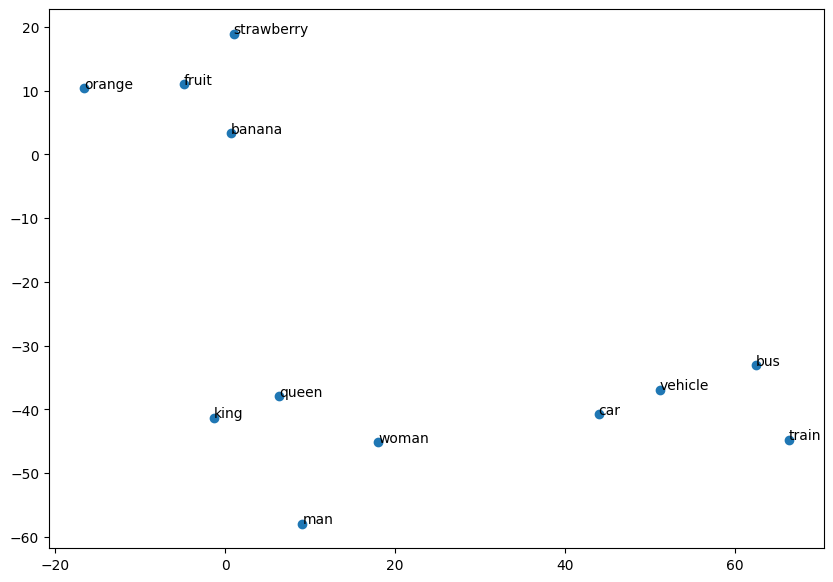
In this example, you will see how words like “car” and “vehicle” or “strawberry” and “orange” are positioned closely in the embedding space, reflecting their semantic similarity.

Example 2: Visualizing Image Embeddings from MNIST with a Convolutional Neural Network (CNN)

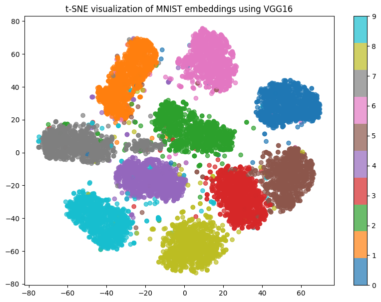
Embeddings are not limited to words—they are also applied to dense data like images. For example, in a convolutional neural network (CNN), the output from the penultimate layer can be treated as the embedding of the image. Let’s use the MNIST dataset (handwritten digits) and a simple CNN model to extract image embeddings and visualize them using t-SNE.

Here’s how you can do this:

import torch
import torch.nn as nn
from torchvision import datasets, transforms, models
from sklearn.manifold import TSNE
import matplotlib.pyplot as plt

# Check if GPU is available and set the device accordingly
device = torch.device("cuda" if torch.cuda.is_available() else "cpu")
print(f'Using device: {device}')

# Define the transformation to convert the MNIST images to 3-channel images and resize them to match VGG input
transform = transforms.Compose([
    transforms.Resize((224, 224)),  # Resize to 224x224, required for VGG16
    transforms.Grayscale(3),  # Convert MNIST 1-channel to 3-channel (RGB)
    transforms.ToTensor(),
    transforms.Normalize(mean=[0.485, 0.456, 0.406], std=[0.229, 0.224, 0.225])
])

# Load the MNIST dataset
test_dataset = datasets.MNIST(root='./data', train=False, transform=transform, download=True)
test_loader = torch.utils.data.DataLoader(test_dataset, batch_size=64, shuffle=False)

# Load a pre-trained VGG16 model
model = models.vgg16(pretrained=True)

# Remove the final classification layer to get embeddings
model = torch.nn.Sequential(*(list(model.children())[:-1]))

# Move the model to the designated device (GPU or CPU)
model = model.to(device)

# Set the model to evaluation mode
model.eval()

# Extract embeddings from the test set
embeddings_list = []
labels_list = []

with torch.no_grad():
    for data, target in test_loader:
        # Move data to the device
        data = data.to(device)
        target = target.to(device)

        # Forward pass through the model to get embeddings
        embeddings = model(data)
        embeddings = embeddings.view(embeddings.size(0), -1)  # Flatten the embeddings
        embeddings_list.append(embeddings.cpu())  # Move embeddings back to CPU for further processing
        labels_list.append(target.cpu())

# Concatenate all embeddings and labels
embeddings = torch.cat(embeddings_list).numpy()
labels = torch.cat(labels_list).numpy()

# Apply t-SNE to reduce the dimensionality of the embeddings to 2D
tsne = TSNE(n_components=2, random_state=42)
reduced_embeddings = tsne.fit_transform(embeddings)

# Visualize the 2D embeddings
plt.figure(figsize=(10, 7))
plt.scatter(reduced_embeddings[:, 0], reduced_embeddings[:, 1], c=labels, cmap='tab10', alpha=0.7)
plt.colorbar()
plt.title('t-SNE visualization of MNIST embeddings using VGG16')
plt.show()

images/cnn_embeddings

This shows how CNNs can generate meaningful embeddings for images, and how t-SNE helps visualize these embeddings in a low-dimensional space.

Latent Space

Latent space is the space in which compressed representations of data reside. Latent vectors, learned by a neural network, are useful for generating new data or reconstructing inputs, as seen in autoencoders.

Example: Programming an Autoencoder and Visualizing Latent Space with MNIST

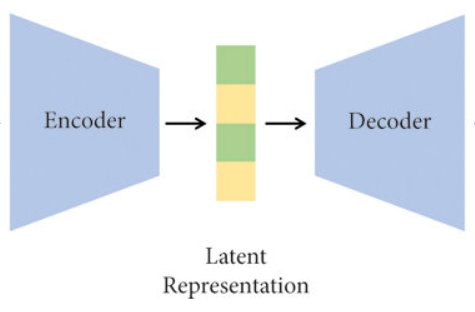
Autoencoders are unsupervised neural networks that learn compressed representations of input data. The bottleneck layer contains the latent representation of the input.

images/autoencoder.PNG

Here’s a simple implementation using PyTorch, training on the MNIST dataset, and visualizing the latent space using t-SNE:

import torch
import torch.nn as nn
import torch.optim as optim
from torchvision import datasets, transforms
from sklearn.manifold import TSNE
import numpy as np
import matplotlib.pyplot as plt

# Check if GPU is available and set the device accordingly
device = torch.device("cuda" if torch.cuda.is_available() else "cpu")
print(f'Using device: {device}')

# Define the Autoencoder
class Autoencoder(nn.Module):
    def __init__(self):
        super(Autoencoder, self).__init__()
        self.encoder = nn.Sequential(
            nn.Linear(784, 128),
            nn.ReLU(),
            nn.Linear(128, 64),
            nn.ReLU(),
            nn.Linear(64, 32)  # Latent space
        )
        self.decoder = nn.Sequential(
            nn.Linear(32, 64),
            nn.ReLU(),
            nn.Linear(64, 128),
            nn.ReLU(),
            nn.Linear(128, 784),
            nn.Sigmoid()  # Output layer
        )
    
    def forward(self, x):
        latent = self.encoder(x)
        reconstructed = self.decoder(latent)
        return reconstructed, latent

# Setup for MNIST dataset
transform = transforms.Compose([
    transforms.ToTensor(),
    transforms.Normalize((0.5,), (0.5,))
])
dataset = datasets.MNIST(root='./data', train=True, download=True, transform=transform)
data_loader = torch.utils.data.DataLoader(dataset, batch_size=32, shuffle=True)

# Initialize the autoencoder and move it to the device
autoencoder = Autoencoder().to(device)
criterion = nn.MSELoss()
optimizer = optim.Adam(autoencoder.parameters(), lr=0.001)

# Train the autoencoder
for epoch in range(10):
    for images, _ in data_loader:
        images = images.view(images.size(0), -1).to(device)  # Flatten images and move to device
        outputs, latents = autoencoder(images)
        loss = criterion(outputs, images)
        optimizer.zero_grad()
        loss.backward()
        optimizer.step()
    print(f'Epoch {epoch+1}, Loss: {loss.item()}')

# Extracting and visualizing the latent space
latent_vectors = []
labels = []

with torch.no_grad():
    for images, targets in data_loader:
        images = images.view(images.size(0), -1).to(device)
        _, latents = autoencoder(images)
        latent_vectors.extend(latents.cpu().detach().numpy())  # Move latents back to CPU for t-SNE
        labels.extend(targets.numpy())

tsne = TSNE(n_components=2, random_state=42)
reduced_latents = tsne.fit_transform(np.array(latent_vectors))

# Visualize the t-SNE of latent space
plt.figure(figsize=(10, 7))
scatter = plt.scatter(reduced_latents[:, 0], reduced_latents[:, 1], c=labels, cmap='tab10', alpha=0.7)
plt.colorbar(scatter)
plt.title('t-SNE visualization of latent space of MNIST digits')
plt.show()

images/autoencoder.PNG

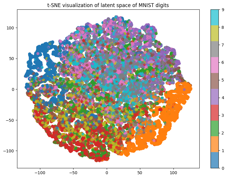
In this example, the latent space is the output of the encoder, which captures essential features of the input while discarding unnecessary information. The autoencoder reconstructs the input from this compressed latent representation.

Representation

A representation is an encoded version of the original input that can take various forms, such as embeddings, latent vectors, or even simple encodings like one-hot vectors.

Example: One-Hot Encoding vs. Learned Representations

While a one-hot vector is a simple representation, embedding methods generate dense, continuous vectors that capture more nuanced relationships between items.

For instance, the following example contrasts a one-hot encoded vector and its embedding:

import torch.nn as nn

# One-hot encoding of a categorical variable with 5 classes
one_hot = torch.eye(5)[[1, 3, 4]]  # Encoding categories 1, 3, 4

# Embedding layer to map one-hot to dense vector
embedding_layer = nn.Embedding(5, 3)  # 5 categories, embedding of size 3
embedding_vectors = embedding_layer(torch.LongTensor([1, 3, 4]))

print("One-hot Encoded Vectors:")
print(one_hot)
print("Embedding Vectors:")
print(embedding_vectors)

Results:

One-hot Encoded Vectors:
tensor([[0., 1., 0., 0., 0.],
        [0., 0., 0., 1., 0.],
        [0., 0., 0., 0., 1.]])
Embedding Vectors:
tensor([[-1.5065,  0.8503,  0.9195],
        [ 1.0450,  0.9560, -0.7647],
        [-1.7090,  0.7112, -1.6332]], grad_fn=<EmbeddingBackward0>)

Here, the one-hot encoded vectors are sparse, while the embedding vectors are dense and continuous, capturing semantic similarities between the categories.

Conclusion

This blog post has explored the fundamental concepts of embeddings, latent spaces, and representations, which are pivotal in the field of deep learning. Embeddings help in reducing high-dimensional data to more manageable, low-dimensional spaces while preserving semantic similarities, crucial for tasks like natural language processing and image recognition. Latent spaces, often encoded by networks like autoencoders, play a crucial role in data compression and denoising, facilitating efficient data reconstruction and generation. Lastly, representations form the backbone of how models perceive and interpret data, influencing their ability to learn and make predictions.

Understanding these concepts not only enhances our comprehension of how deep learning models function but also improves our ability to develop more sophisticated and efficient AI systems. Whether in academic research or practical applications, the ability to effectively manipulate data representations can lead to significant breakthroughs in technology and science.

References:

Bengio, Y., Courville, A., & Vincent, P. (2013). “Representation Learning: A Review and New Perspectives.” IEEE Transactions on Pattern Analysis and Machine Intelligence, 35(8), 1798-1828. Link
Mikolov, T., Chen, K., Corrado, G., & Dean, J. (2013). “Efficient Estimation of Word Representations in Vector Space.” arXiv preprint arXiv:1301.3781. Link
Goodfellow, I., Bengio, Y., & Courville, A. (2016). “Deep Learning.” MIT Press. This book provides comprehensive coverage on the theory and applications of deep learning, including a detailed discussion on representations. Link